Reading data from the web
In data import, we saw how to load data from a variety of formats; this is a fairly standard way to get data that have been gathered as part of a study. In a lot of cases, though, you’re going to have to go out and get the data you want or need. That’s what we’re covering now.
This is the first module in the Data Wrangling II topic.
Overview
Learning Objectives
Gather data from online sources (i.e. “scrape”) using APIs, rvest, and httr.
Video Lecture
Example
As always, I’ll create a new GH Repo + local project called
data_wrangling_ii, and open a new R Markdown file called
reading_data_from_the_web.Rmd. Although we’ll mostly be
getting data from the web, we’ll revisit some of these examples, so I’ll
create a data subdirectory and put those in it.
There are some new additions to our standard packages
(rvest and httr); I’m loading everything we
need now. Now’s also the time to “install” the Selector Gadget.
library(tidyverse)
library(rvest)
library(httr)
Extracting tables
This page contains data from the National Survey on Drug Use and Health; it includes tables for drug use in the past year or month, separately for specific kinds of drug use. These data are potentially useful for analysis, and we’d like to be able to read in the first table.
First, let’s make sure we can load the data from the web.
url = "http://samhda.s3-us-gov-west-1.amazonaws.com/s3fs-public/field-uploads/2k15StateFiles/NSDUHsaeShortTermCHG2015.htm"
drug_use_html = read_html(url)

drug_use_html
## {html_document}
## <html lang="en">
## [1] <head>\n<link rel="P3Pv1" href="http://www.samhsa.gov/w3c/p3p.xml">\n<tit ...
## [2] <body>\r\n\r\n<noscript>\r\n<p>Your browser's Javascript is off. Hyperlin ...Doesn’t look like much, but we’re there. Rather than trying to grab something using a CSS selector, let’s try our luck extracting the tables from the HTML.
drug_use_html |>
  html_table()
## [[1]]
## # A tibble: 57 × 16
## State `12+(2013-2014)` `12+(2014-2015)` `12+(P Value)` `12-17(2013-2014)`
## <chr> <chr> <chr> <chr> <chr>
## 1 "NOTE: S… "NOTE: State an… "NOTE: State an… "NOTE: State … "NOTE: State and …
## 2 "Total U… "12.90a" "13.36" "0.002" "13.28b"
## 3 "Northea… "13.88a" "14.66" "0.005" "13.98"
## 4 "Midwest" "12.40b" "12.76" "0.082" "12.45"
## 5 "South" "11.24a" "11.64" "0.029" "12.02"
## 6 "West" "15.27" "15.62" "0.262" "15.53a"
## 7 "Alabama" "9.98" "9.60" "0.426" "9.90"
## 8 "Alaska" "19.60a" "21.92" "0.010" "17.30"
## 9 "Arizona" "13.69" "13.12" "0.364" "15.12"
## 10 "Arkansa… "11.37" "11.59" "0.678" "12.79"
## # ℹ 47 more rows
## # ℹ 11 more variables: `12-17(2014-2015)` <chr>, `12-17(P Value)` <chr>,
## # `18-25(2013-2014)` <chr>, `18-25(2014-2015)` <chr>, `18-25(P Value)` <chr>,
## # `26+(2013-2014)` <chr>, `26+(2014-2015)` <chr>, `26+(P Value)` <chr>,
## # `18+(2013-2014)` <chr>, `18+(2014-2015)` <chr>, `18+(P Value)` <chr>
##
## [[2]]
## # A tibble: 57 × 16
## State `12+(2013-2014)` `12+(2014-2015)` `12+(P Value)` `12-17(2013-2014)`
## <chr> <chr> <chr> <chr> <chr>
## 1 "NOTE: S… "NOTE: State an… "NOTE: State an… "NOTE: State … "NOTE: State and …
## 2 "Total U… "7.96a" "8.34" "0.001" "7.22"
## 3 "Northea… "8.58a" "9.28" "0.001" "7.68"
## 4 "Midwest" "7.50a" "7.92" "0.009" "6.64"
## 5 "South" "6.74a" "7.02" "0.044" "6.31"
## 6 "West" "9.84" "10.08" "0.324" "8.85"
## 7 "Alabama" "5.57" "5.35" "0.510" "4.98"
## 8 "Alaska" "11.85a" "14.38" "0.002" "9.19"
## 9 "Arizona" "8.80" "8.51" "0.570" "8.30"
## 10 "Arkansa… "6.70" "7.17" "0.240" "6.22"
## # ℹ 47 more rows
## # ℹ 11 more variables: `12-17(2014-2015)` <chr>, `12-17(P Value)` <chr>,
## # `18-25(2013-2014)` <chr>, `18-25(2014-2015)` <chr>, `18-25(P Value)` <chr>,
## # `26+(2013-2014)` <chr>, `26+(2014-2015)` <chr>, `26+(P Value)` <chr>,
## # `18+(2013-2014)` <chr>, `18+(2014-2015)` <chr>, `18+(P Value)` <chr>
##
## [[3]]
## # A tibble: 57 × 16
## State `12+(2013-2014)` `12+(2014-2015)` `12+(P Value)` `12-17(2013-2014)`
## <chr> <chr> <chr> <chr> <chr>
## 1 "NOTE: S… "NOTE: State an… "NOTE: State an… "NOTE: State … "NOTE: State and …
## 2 "Total U… "1.91" "1.95" "0.276" "5.60"
## 3 "Northea… "2.01" "2.04" "0.634" "5.85b"
## 4 "Midwest" "1.95" "1.96" "0.854" "5.31"
## 5 "South" "1.69" "1.75" "0.137" "5.18"
## 6 "West" "2.20" "2.21" "0.868" "6.37b"
## 7 "Alabama" "1.42" "1.49" "0.383" "4.46"
## 8 "Alaska" "3.01a" "3.54" "0.012" "6.99"
## 9 "Arizona" "2.16" "2.15" "0.934" "6.58"
## 10 "Arkansa… "1.82" "1.84" "0.794" "5.78"
## # ℹ 47 more rows
## # ℹ 11 more variables: `12-17(2014-2015)` <chr>, `12-17(P Value)` <chr>,
## # `18-25(2013-2014)` <chr>, `18-25(2014-2015)` <chr>, `18-25(P Value)` <chr>,
## # `26+(2013-2014)` <chr>, `26+(2014-2015)` <chr>, `26+(P Value)` <chr>,
## # `18+(2013-2014)` <chr>, `18+(2014-2015)` <chr>, `18+(P Value)` <chr>
##
## [[4]]
## # A tibble: 57 × 16
## State `12+(2013-2014)` `12+(2014-2015)` `12+(P Value)` `12-17(2013-2014)`
## <chr> <chr> <chr> <chr> <chr>
## 1 "NOTE: S… "NOTE: State an… "NOTE: State an… "NOTE: State … "NOTE: State and …
## 2 "Total U… "1.66a" "1.76" "0.040" "0.60"
## 3 "Northea… "1.94a" "2.18" "0.012" "0.60"
## 4 "Midwest" "1.37" "1.43" "0.282" "0.48"
## 5 "South" "1.45b" "1.56" "0.067" "0.53"
## 6 "West" "2.03" "2.05" "0.816" "0.82"
## 7 "Alabama" "1.23" "1.22" "0.995" "0.42"
## 8 "Alaska" "1.54a" "2.00" "0.010" "0.51"
## 9 "Arizona" "2.25" "2.29" "0.861" "1.01"
## 10 "Arkansa… "0.93" "1.07" "0.208" "0.41"
## # ℹ 47 more rows
## # ℹ 11 more variables: `12-17(2014-2015)` <chr>, `12-17(P Value)` <chr>,
## # `18-25(2013-2014)` <chr>, `18-25(2014-2015)` <chr>, `18-25(P Value)` <chr>,
## # `26+(2013-2014)` <chr>, `26+(2014-2015)` <chr>, `26+(P Value)` <chr>,
## # `18+(2013-2014)` <chr>, `18+(2014-2015)` <chr>, `18+(P Value)` <chr>
##
## [[5]]
## # A tibble: 57 × 16
## State `12+(2013-2014)` `12+(2014-2015)` `12+(P Value)` `12-17(2013-2014)`
## <chr> <chr> <chr> <chr> <chr>
## 1 "NOTE: S… "NOTE: State an… "NOTE: State an… "NOTE: State … "NOTE: State and …
## 2 "Total U… "0.30" "0.33" "0.217" "0.12"
## 3 "Northea… "0.43a" "0.54" "0.007" "0.13"
## 4 "Midwest" "0.30" "0.31" "0.638" "0.11"
## 5 "South" "0.27" "0.26" "0.444" "0.12"
## 6 "West" "0.25" "0.29" "0.152" "0.13"
## 7 "Alabama" "0.22" "0.27" "0.171" "0.10"
## 8 "Alaska" "0.70a" "1.23" "0.044" "0.11"
## 9 "Arizona" "0.32a" "0.55" "0.001" "0.17"
## 10 "Arkansa… "0.19" "0.17" "0.398" "0.10"
## # ℹ 47 more rows
## # ℹ 11 more variables: `12-17(2014-2015)` <chr>, `12-17(P Value)` <chr>,
## # `18-25(2013-2014)` <chr>, `18-25(2014-2015)` <chr>, `18-25(P Value)` <chr>,
## # `26+(2013-2014)` <chr>, `26+(2014-2015)` <chr>, `26+(P Value)` <chr>,
## # `18+(2013-2014)` <chr>, `18+(2014-2015)` <chr>, `18+(P Value)` <chr>
##
## [[6]]
## # A tibble: 57 × 16
## State `12+(2013-2014)` `12+(2014-2015)` `12+(P Value)` `12-17(2013-2014)`
## <chr> <chr> <chr> <chr> <chr>
## 1 "NOTE: S… "NOTE: State an… "NOTE: State an… "NOTE: State … "NOTE: State and …
## 2 "Total U… "52.42" "52.18" "0.337" "11.55a"
## 3 "Northea… "57.80a" "56.66" "0.009" "13.19"
## 4 "Midwest" "55.14a" "54.36" "0.032" "11.31a"
## 5 "South" "48.74" "48.85" "0.759" "10.87a"
## 6 "West" "51.67" "52.07" "0.383" "11.71a"
## 7 "Alabama" "44.72" "43.94" "0.533" "10.53a"
## 8 "Alaska" "54.02" "54.98" "0.444" "9.22"
## 9 "Arizona" "51.80" "51.19" "0.613" "11.90b"
## 10 "Arkansa… "42.45" "41.81" "0.588" "9.90"
## # ℹ 47 more rows
## # ℹ 11 more variables: `12-17(2014-2015)` <chr>, `12-17(P Value)` <chr>,
## # `18-25(2013-2014)` <chr>, `18-25(2014-2015)` <chr>, `18-25(P Value)` <chr>,
## # `26+(2013-2014)` <chr>, `26+(2014-2015)` <chr>, `26+(P Value)` <chr>,
## # `18+(2013-2014)` <chr>, `18+(2014-2015)` <chr>, `18+(P Value)` <chr>
##
## [[7]]
## # A tibble: 57 × 4
## State Alcohol Use inPast M…¹ Alcohol Use inPast M…² Alcohol Use inPast M…³
## <chr> <chr> <chr> <chr>
## 1 "NOTE: … "NOTE: State and cens… "NOTE: State and cens… "NOTE: State and cens…
## 2 "Total … "22.76a" "21.57" "0.000"
## 3 "Northe… "26.11" "25.98" "0.792"
## 4 "Midwes… "23.73a" "22.00" "0.000"
## 5 "South" "20.68a" "19.66" "0.010"
## 6 "West" "22.73a" "21.01" "0.000"
## 7 "Alabam… "19.25" "18.19" "0.305"
## 8 "Alaska" "21.47b" "23.91" "0.058"
## 9 "Arizon… "22.01a" "19.25" "0.009"
## 10 "Arkans… "18.07" "16.65" "0.106"
## # ℹ 47 more rows
## # ℹ abbreviated names: ¹`Alcohol Use inPast Month(2013-2014)`,
## # ²`Alcohol Use inPast Month(2014-2015)`,
## # ³`Alcohol Use inPast Month(P Value)`
##
## [[8]]
## # A tibble: 57 × 16
## State `12+(2013-2014)` `12+(2014-2015)` `12+(P Value)` `12-17(2013-2014)`
## <chr> <chr> <chr> <chr> <chr>
## 1 "NOTE: S… "NOTE: State an… "NOTE: State an… "NOTE: State … "NOTE: State and …
## 2 "Total U… "25.36a" "24.56" "0.000" "7.42a"
## 3 "Northea… "23.76" "23.30" "0.216" "7.18a"
## 4 "Midwest" "28.57a" "27.39" "0.000" "8.58a"
## 5 "South" "26.91a" "26.24" "0.034" "7.57a"
## 6 "West" "21.20a" "20.29" "0.015" "6.31a"
## 7 "Alabama" "31.62" "30.46" "0.295" "8.43"
## 8 "Alaska" "29.30a" "31.51" "0.048" "10.73"
## 9 "Arizona" "22.14" "22.51" "0.678" "6.81"
## 10 "Arkansa… "35.57" "34.05" "0.188" "10.89"
## # ℹ 47 more rows
## # ℹ 11 more variables: `12-17(2014-2015)` <chr>, `12-17(P Value)` <chr>,
## # `18-25(2013-2014)` <chr>, `18-25(2014-2015)` <chr>, `18-25(P Value)` <chr>,
## # `26+(2013-2014)` <chr>, `26+(2014-2015)` <chr>, `26+(P Value)` <chr>,
## # `18+(2013-2014)` <chr>, `18+(2014-2015)` <chr>, `18+(P Value)` <chr>
##
## [[9]]
## # A tibble: 57 × 16
## State `12+(2013-2014)` `12+(2014-2015)` `12+(P Value)` `12-17(2013-2014)`
## <chr> <chr> <chr> <chr> <chr>
## 1 "NOTE: S… "NOTE: State an… "NOTE: State an… "NOTE: State … "NOTE: State and …
## 2 "Total U… "21.05a" "20.12" "0.000" "5.24a"
## 3 "Northea… "19.69" "19.13" "0.101" "5.10a"
## 4 "Midwest" "23.84a" "22.50" "0.000" "6.16a"
## 5 "South" "22.37a" "21.41" "0.001" "5.22a"
## 6 "West" "17.43a" "16.66" "0.026" "4.56a"
## 7 "Alabama" "25.90" "24.25" "0.106" "5.66"
## 8 "Alaska" "22.00a" "24.64" "0.008" "6.15"
## 9 "Arizona" "18.73" "19.23" "0.576" "4.95"
## 10 "Arkansa… "28.51" "27.81" "0.519" "7.13"
## # ℹ 47 more rows
## # ℹ 11 more variables: `12-17(2014-2015)` <chr>, `12-17(P Value)` <chr>,
## # `18-25(2013-2014)` <chr>, `18-25(2014-2015)` <chr>, `18-25(P Value)` <chr>,
## # `26+(2013-2014)` <chr>, `26+(2014-2015)` <chr>, `26+(P Value)` <chr>,
## # `18+(2013-2014)` <chr>, `18+(2014-2015)` <chr>, `18+(P Value)` <chr>
##
## [[10]]
## # A tibble: 57 × 16
## State `12+(2013-2014)` `12+(2014-2015)` `12+(P Value)` `12-17(2013-2014)`
## <chr> <chr> <chr> <chr> <chr>
## 1 "NOTE: S… "NOTE: State an… "NOTE: State an… "NOTE: State … "NOTE: State and …
## 2 "Total U… "6.50a" "6.14" "0.001" "2.76"
## 3 "Northea… "6.64" "6.39" "0.193" "2.88"
## 4 "Midwest" "6.59a" "6.25" "0.033" "2.70"
## 5 "South" "6.20a" "5.76" "0.003" "2.65"
## 6 "West" "6.80" "6.47" "0.120" "2.91"
## 7 "Alabama" "5.76a" "4.64" "0.007" "2.84b"
## 8 "Alaska" "6.72" "7.43" "0.153" "2.12"
## 9 "Arizona" "7.60b" "6.66" "0.062" "3.37"
## 10 "Arkansa… "5.23" "4.88" "0.347" "2.63"
## # ℹ 47 more rows
## # ℹ 11 more variables: `12-17(2014-2015)` <chr>, `12-17(P Value)` <chr>,
## # `18-25(2013-2014)` <chr>, `18-25(2014-2015)` <chr>, `18-25(P Value)` <chr>,
## # `26+(2013-2014)` <chr>, `26+(2014-2015)` <chr>, `26+(P Value)` <chr>,
## # `18+(2013-2014)` <chr>, `18+(2014-2015)` <chr>, `18+(P Value)` <chr>
##
## [[11]]
## # A tibble: 57 × 16
## State `12+(2013-2014)` `12+(2014-2015)` `12+(P Value)` `12-17(2013-2014)`
## <chr> <chr> <chr> <chr> <chr>
## 1 "NOTE: S… "NOTE: State an… "NOTE: State an… "NOTE: State … "NOTE: State and …
## 2 "Total U… "3.04" "2.97" "0.321" "1.01"
## 3 "Northea… "3.01" "3.09" "0.500" "1.02"
## 4 "Midwest" "3.06b" "2.86" "0.061" "1.03"
## 5 "South" "2.92a" "2.73" "0.047" "0.96"
## 6 "West" "3.25" "3.37" "0.409" "1.05"
## 7 "Alabama" "2.99a" "2.34" "0.026" "0.98"
## 8 "Alaska" "3.21" "3.67" "0.200" "0.77"
## 9 "Arizona" "3.44" "3.62" "0.591" "1.11"
## 10 "Arkansa… "2.73" "2.42" "0.255" "0.96"
## # ℹ 47 more rows
## # ℹ 11 more variables: `12-17(2014-2015)` <chr>, `12-17(P Value)` <chr>,
## # `18-25(2013-2014)` <chr>, `18-25(2014-2015)` <chr>, `18-25(P Value)` <chr>,
## # `26+(2013-2014)` <chr>, `26+(2014-2015)` <chr>, `26+(P Value)` <chr>,
## # `18+(2013-2014)` <chr>, `18+(2014-2015)` <chr>, `18+(P Value)` <chr>
##
## [[12]]
## # A tibble: 57 × 10
## State `18+(2013-2014)` `18+(2014-2015)` `18+(P Value)` `18-25(2013-2014)`
## <chr> <chr> <chr> <chr> <chr>
## 1 "NOTE: S… "NOTE: State an… "NOTE: State an… "NOTE: State … "NOTE: State and …
## 2 "Total U… "4.15" "4.05" "0.325" "4.52a"
## 3 "Northea… "3.93" "3.94" "0.953" "4.67a"
## 4 "Midwest" "4.45" "4.36" "0.511" "4.93a"
## 5 "South" "4.17" "4.00" "0.206" "4.18a"
## 6 "West" "4.02" "3.96" "0.681" "4.56b"
## 7 "Alabama" "4.53" "4.64" "0.749" "4.30"
## 8 "Alaska" "3.90" "4.02" "0.707" "4.60a"
## 9 "Arizona" "4.09" "4.33" "0.491" "4.45"
## 10 "Arkansa… "5.24" "5.27" "0.942" "4.49"
## # ℹ 47 more rows
## # ℹ 5 more variables: `18-25(2014-2015)` <chr>, `18-25(P Value)` <chr>,
## # `26+(2013-2014)` <chr>, `26+(2014-2015)` <chr>, `26+(P Value)` <chr>
##
## [[13]]
## # A tibble: 57 × 10
## State `18+(2013-2014)` `18+(2014-2015)` `18+(P Value)` `18-25(2013-2014)`
## <chr> <chr> <chr> <chr> <chr>
## 1 "NOTE: S… "NOTE: State an… "NOTE: State an… "NOTE: State … "NOTE: State and …
## 2 "Total U… "18.29" "18.01" "0.146" "19.75a"
## 3 "Northea… "17.87" "17.76" "0.735" "20.80a"
## 4 "Midwest" "18.61" "18.34" "0.356" "20.45a"
## 5 "South" "18.01" "17.82" "0.519" "18.22a"
## 6 "West" "18.79b" "18.18" "0.088" "20.70a"
## 7 "Alabama" "19.51" "18.85" "0.469" "18.09"
## 8 "Alaska" "18.12" "18.11" "0.989" "20.33a"
## 9 "Arizona" "18.59" "18.32" "0.756" "18.76"
## 10 "Arkansa… "20.00" "19.77" "0.816" "19.99"
## # ℹ 47 more rows
## # ℹ 5 more variables: `18-25(2014-2015)` <chr>, `18-25(P Value)` <chr>,
## # `26+(2013-2014)` <chr>, `26+(2014-2015)` <chr>, `26+(P Value)` <chr>
##
## [[14]]
## # A tibble: 57 × 10
## State `18+(2013-2014)` `18+(2014-2015)` `18+(P Value)` `18-25(2013-2014)`
## <chr> <chr> <chr> <chr> <chr>
## 1 "NOTE: S… "NOTE: State an… "NOTE: State an… "NOTE: State … "NOTE: State and …
## 2 "Total U… "3.94" "3.99" "0.526" "7.44a"
## 3 "Northea… "3.81" "3.93" "0.407" "7.60b"
## 4 "Midwest" "4.11" "4.14" "0.791" "7.83"
## 5 "South" "3.84" "3.86" "0.896" "6.89a"
## 6 "West" "4.02" "4.12" "0.522" "7.84"
## 7 "Alabama" "3.98" "4.02" "0.885" "7.31"
## 8 "Alaska" "4.21" "4.68" "0.237" "8.30b"
## 9 "Arizona" "4.23" "4.34" "0.775" "7.04"
## 10 "Arkansa… "4.58" "4.41" "0.682" "6.67"
## # ℹ 47 more rows
## # ℹ 5 more variables: `18-25(2014-2015)` <chr>, `18-25(P Value)` <chr>,
## # `26+(2013-2014)` <chr>, `26+(2014-2015)` <chr>, `26+(P Value)` <chr>
##
## [[15]]
## # A tibble: 57 × 13
## State `18+(2013-2014)` `18+(2014-2015)` `18+(P Value)` `12-17(2013-2014)`
## <chr> <chr> <chr> <chr> <chr>
## 1 "NOTE: S… "NOTE: State an… "NOTE: State an… "NOTE: State … "NOTE: State and …
## 2 "Total U… "6.63" "6.64" "0.915" "11.01a"
## 3 "Northea… "6.66" "6.82" "0.458" "10.63a"
## 4 "Midwest" "6.81" "6.87" "0.736" "10.81a"
## 5 "South" "6.47" "6.52" "0.750" "10.77a"
## 6 "West" "6.67" "6.47" "0.353" "11.82a"
## 7 "Alabama" "6.85" "6.81" "0.948" "10.74"
## 8 "Alaska" "6.57" "6.73" "0.770" "9.92a"
## 9 "Arizona" "7.32" "6.77" "0.362" "13.23"
## 10 "Arkansa… "7.31" "7.78" "0.446" "11.95"
## # ℹ 47 more rows
## # ℹ 8 more variables: `12-17(2014-2015)` <chr>, `12-17(P Value)` <chr>,
## # `18-25(2013-2014)` <chr>, `18-25(2014-2015)` <chr>, `18-25(P Value)` <chr>,
## # `26+(2013-2014)` <chr>, `26+(2014-2015)` <chr>, `26+(P Value)` <chr>This has extracted all of the tables on the original page; that’s why we have a list with 15 elements. (We haven’t really talked about lists yet, but for now you can think of them as a general collection of objects in R. As we proceed, syntax for extracting individual elements from a list will become clear, and we’ll talk lots about lists in list columns.)
We’re only focused on the first table for now, so let’s get the contents from the first list element.
table_marj =
  drug_use_html |>
  html_table() |>
  first()
I won’t print the table here, but if you look at it you’ll notice a problem: the “note” at the bottom of the table appears in every column in the first row. We need to remove that…
table_marj =
  drug_use_html |>
  html_table() |>
  first() |>
  slice(-1)

table_marj
## # A tibble: 56 × 16
## State `12+(2013-2014)` `12+(2014-2015)` `12+(P Value)` `12-17(2013-2014)`
## <chr> <chr> <chr> <chr> <chr>
## 1 Total U.… 12.90a 13.36 0.002 13.28b
## 2 Northeast 13.88a 14.66 0.005 13.98
## 3 Midwest 12.40b 12.76 0.082 12.45
## 4 South 11.24a 11.64 0.029 12.02
## 5 West 15.27 15.62 0.262 15.53a
## 6 Alabama 9.98 9.60 0.426 9.90
## 7 Alaska 19.60a 21.92 0.010 17.30
## 8 Arizona 13.69 13.12 0.364 15.12
## 9 Arkansas 11.37 11.59 0.678 12.79
## 10 Californ… 14.49 15.25 0.103 15.03
## # ℹ 46 more rows
## # ℹ 11 more variables: `12-17(2014-2015)` <chr>, `12-17(P Value)` <chr>,
## # `18-25(2013-2014)` <chr>, `18-25(2014-2015)` <chr>, `18-25(P Value)` <chr>,
## # `26+(2013-2014)` <chr>, `26+(2014-2015)` <chr>, `26+(P Value)` <chr>,
## # `18+(2013-2014)` <chr>, `18+(2014-2015)` <chr>, `18+(P Value)` <chr>Success!! At least, mostly. These data aren’t tidy, but we’ll worry about that soon.
Learning assessment: Create a data frame that contains the cost of living table for New York from this page.
Solution
The code below shows one approach to this data cleaning process:
nyc_cost =
  read_html("https://www.bestplaces.net/cost_of_living/city/new_york/new_york") |>
  html_table(header = TRUE) |>
  first()
In case you hadn’t known, NYC is kind of expensive.
CSS Selectors
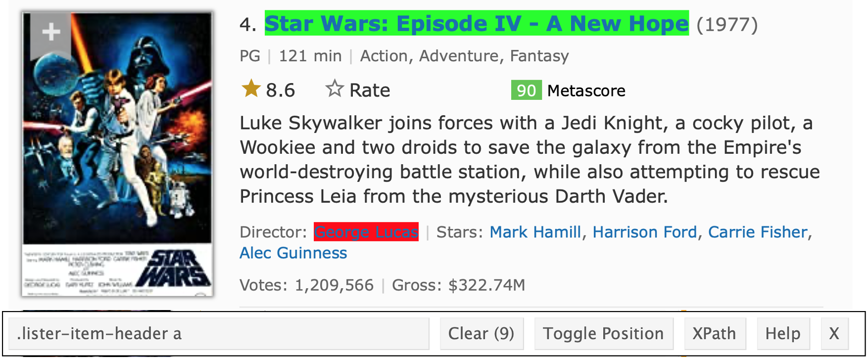
Suppose we’d like to scrape the data about the Star Wars Movies from the IMDB page. The first step is the same as before – we need to get the HTML.
swm_html =
  read_html("https://www.imdb.com/list/ls070150896/")
The information isn’t stored in a handy table, so we’re going to isolate the CSS selector for elements we care about. A bit of clicking around gets me something like below.
For each element, I’ll use the CSS selector in
html_elements() to extract the relevant HTML code, and
convert it to text. Then I can combine these into a data frame.
title_vec =
  swm_html |>
  html_elements(".ipc-title-link-wrapper .ipc-title__text") |>
  html_text()

metascore_vec =
  swm_html |>
  html_elements(".metacritic-score-box") |>
  html_text()

runtime_vec =
  swm_html |>
  html_elements(".dli-title-metadata-item:nth-child(2)") |>
  html_text()

swm_df =
  tibble(
    title = title_vec,
    score = metascore_vec,
    runtime = runtime_vec)
Not everyone loved the prequels …
Learning Assessment: This page contains some (made up) books. Use a process similar to the one above to extract the book titles, stars, and prices.
Solution
The code below will give me relevant information for the books on this page:
url = "http://books.toscrape.com"

books_html = read_html(url)

books_titles =
  books_html |>
  html_elements("h3") |>
  html_text2()

books_stars =
  books_html |>
  html_elements(".star-rating") |>
  html_attr("class")

books_price =
  books_html |>
  html_elements(".price_color") |>
  html_text()

books = tibble(
  title = books_titles,
  stars = books_stars,
  price = books_price
)
Using an API
New York City has a great open data resource, and we’ll use that for our API examples. Although most (all?) of these datasets can be accessed by clicking through a website, we’ll access them directly using the API to improve reproducibility and make it easier to update results to reflect new data.
As a simple example, this page is about a dataset for annual water consumption in NYC, along with the population in that year. First, we’ll import this as a CSV and parse it.
nyc_water =
  GET("https://data.cityofnewyork.us/resource/ia2d-e54m.csv") |>
  content("parsed")
## Rows: 65 Columns: 4
## ── Column specification ────────────────────────────────────────────────────────
## Delimiter: ","
## dbl (4): year, new_york_city_population, nyc_consumption_million_gallons_per...
##
## ℹ Use `spec()` to retrieve the full column specification for this data.
## ℹ Specify the column types or set `show_col_types = FALSE` to quiet this message.We can also import this dataset as a JSON file. This takes a bit more work (and this is, really, a pretty easy case), but it’s still doable.
nyc_water =
  GET("https://data.cityofnewyork.us/resource/ia2d-e54m.json") |>
  content("text") |>
  jsonlite::fromJSON() |>
  as_tibble()
Data.gov also has a lot of data available using their API; often this is available as CSV or JSON as well. For example, we might be interested in data coming from BRFSS. This is importable via the API as a CSV (JSON, in this example, is more complicated).
However, in recent years data.gov has required registration and a
token to keep track of requests. You can find the sign-up (and sign-in)
process in the API
Documentation; the process for creating an account and token is
pretty easy here. Once you have a (public) token, you can include it
through the app_token field that refines the query sent to
the API.
brfss_smart2010 =
  GET("https://chronicdata.cdc.gov/api/v3/views/acme-vg9e/query.csv",
      query = list("app_token" = "ZZ")) |>
  content("parsed")
There are a lot of other potentially useful ways of modifying your API request through the query specification – looking around the website describing the API can be helpful, for example, if the API limits the amount of data you can request by default. In cases like that, to get the full data, you could increase the default amount so that you get all the data at once or you could try iterating over chunks of a few thousand rows.
The use of API tokens is also relatively common. Here, the accounts are free and easy to use, but getting data from Amazon or Twitter is typically harder (and more expensive).
Both the NYC Water and BRFSS examples are, actually, pretty easy – we accessed data that is essentially a data table, and we had a very straightforward API (although updating queries isn’t obvious at first).
To get a sense of how this becomes complicated, let’s look at the Pokemon API (which is also pretty nice).
poke =
  GET("http://pokeapi.co/api/v2/pokemon/1") |>
  content()

poke[["name"]]
## [1] "bulbasaur"poke[["height"]]## [1] 7poke[["abilities"]]## [[1]]
## [[1]]$ability
## [[1]]$ability$name
## [1] "overgrow"
##
## [[1]]$ability$url
## [1] "https://pokeapi.co/api/v2/ability/65/"
##
##
## [[1]]$is_hidden
## [1] FALSE
##
## [[1]]$slot
## [1] 1
##
##
## [[2]]
## [[2]]$ability
## [[2]]$ability$name
## [1] "chlorophyll"
##
## [[2]]$ability$url
## [1] "https://pokeapi.co/api/v2/ability/34/"
##
##
## [[2]]$is_hidden
## [1] TRUE
##
## [[2]]$slot
## [1] 3To build a Pokemon dataset for analysis, you’d need to distill the data returned from the API into a useful format; iterate across all pokemon; and combine the results.
For both of the API examples we saw today, it wouldn’t be terrible to just download the CSV, document where it came from carefully, and move on. APIs are more helpful when the full dataset is complex and you only need pieces, or when the data are updated regularly.
Be reasonable
When you’re reading data from the web, remember you’re accessing resources on someone else’s server – either by reading HTML or by accessing data via an API. In some cases, those who make data public will take steps to limit bandwidth devoted to a small number of users. Amazon and IMDB, for example, probably won’t notice if you scrape small amounts of data but would notice if you tried to read data from thousands of pages every time you knitted a document.
Similarly, API developers can (and will) limit the number of database
entries that can be accessed in a single request. In those cases you’d
have to take some steps to iterate over “pages” and combine the results;
as an example, our code for the NYC Restaurant
Inspections does this. In some cases, API developers protect
themselves from unreasonable use by requiring users to be authenticated
– it’s still possible to use httr in these cases, but we
won’t get into it.
Other materials
- A recent short course presented similar topics to those above; a GitHub repo for the course is here
- A lot of NYC data is public; this is a good place to start looking for interesting data
- There are some cool projects based on scraped data; the RStudio community collected some here
- Check out the R
file used to create the
starwarsdataset (in thetidyverse) using the Star Wars API (from the maker of the Pokemon API). - Some really helpful R packages are wrappers for APIs – the
rnoaapackage we’ve used is an example, and so isrtweet
The code that I produced working examples in lecture is here.